📈 Demand Planning makes Croston, XGBoost signals, and naive fallback GA
📈 Demand Planning makes Croston, XGBoost signals, and naive fallback GA
Microsoft has removed the preview label from three Demand Planning forecasting capabilities: Croston’s method for intermittent demand, naive forecasting for short series, and XGBoost forecasts that combine demand with up to five external signals.
These aren’t three new algorithms. They were available in earlier app versions, but the change published on October 23, 2026 moves them out of preview terms and makes production adoption possible under the product’s normal terms. General availability doesn’t remove their entry conditions or turn automatic selection into an accuracy guarantee.
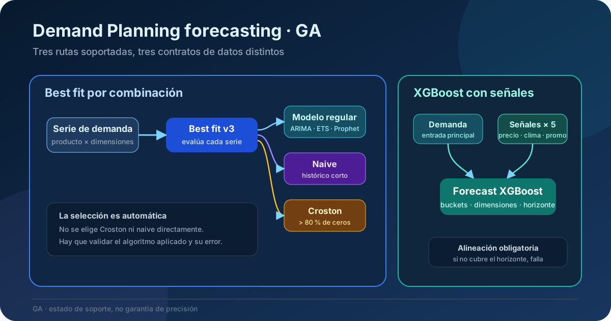
Original diagram. Best fit decides per dimension combination when to use a fallback; XGBoost combines one primary input with aligned signals.
What changed
The official change removes preview notices from the documentation and updates the Best fit model version catalog:
| Capability | Path | Documented requirement | Purpose |
|---|---|---|---|
| Naive forecasting | Best fit model - version 2 or later | Demand Planning 1.0.0.3424 or later | Fallback when data is scarce and no seasonality is detected |
| Croston’s method | Best fit model - version 3 or later | Demand Planning 1.1.0.4 or later | Fallback for nonseasonal series with more than 80% zero values |
| Forecast with signals | Forecast with signals step | Feature introduced in Demand Planning 1.1 | XGBoost with one primary series and up to five signals |
GA changes support status, not the functional architecture. Existing models aren’t automatically migrated from Best fit v1 to v2 or v3, and a Forecast step doesn’t become Forecast with signals. You must explicitly select and test the appropriate path.
How Best fit chooses between a regular model and a fallback
Best fit model evaluates each product and dimension combination separately. A single run can therefore use a regular statistical model for some combinations and a fallback for others.
Naive forecasting for short series
Naive forecasting applies only when Best fit model - version 2 or later is used, automatic seasonality detection is enabled, no seasonal pattern is detected, and the dataset contains fewer than twice the applicable threshold:
| Granularity | Threshold | Low-data range |
|---|---|---|
| Day | 14 points | Fewer than 28 points |
| Week | 12 points | Fewer than 24 points |
| Month | 12 points | Fewer than 24 points |
Within that range, behavior varies by volume:
- below half the threshold: copy the data and fill with zeros;
- between half and the threshold: copy and use linear interpolation;
- between the threshold and twice the threshold: use an averaged copy.
You can’t select naive forecasting directly. It’s a controlled fallback when there isn’t enough information to train a regular model. If it appears across many combinations, treat that as a signal that historical depth or quality may be insufficient.
Croston for intermittent demand
Croston is evaluated with Best fit model - version 3 or later and applies when all these conditions are met:
- the series doesn’t meet the naive forecasting conditions;
- there is no clear seasonal pattern;
- more than 80% of input values are zero.
The method separates two phenomena: average demand size when demand occurs and the average interval between events. This prevents a long run of zeros from forcing an all-zero forecast or a single spike from creating an artificial trend.
The 80% boundary is a product rule, not a published configurable parameter. Don’t manipulate zeros, aggregation, or granularity just to force selection. First establish whether zero truly means no demand rather than missing data.
Forecast with signals is a separate path
Signal forecasting isn’t part of the Best fit selector. The Forecast with signals step always uses XGBoost and requires a model with parallel branches:
- one branch starts with the primary series, such as historical sales;
- one to five branches start with Signal steps, such as price, promotions, inflation, or weather;
- each branch can contain transformations;
- all branches converge into Forecast with signals;
- the result ends in a Save step.
General availability doesn’t relax alignment rules:
- time bucket sizes must be compatible;
- dimensions used for alignment must match;
- signals must cover the training history you intend to use and extend through the forecast horizon;
- if a signal starts later, older primary history is ignored;
- if it doesn’t reach the end of the horizon, the run fails.
The model supports up to five signals, not five columns. Each signal is a time series with its own branch and dimension contract.
Step-by-step implementation
1. Confirm the installed version and current model
Check the installed Demand Planning version before editing profiles. Naive forecasting requires at least 1.0.0.3424; Croston requires 1.1.0.4. If a model remains on Best fit version 1, removal of the preview label doesn’t change its behavior.
Export or document the current configuration and record a baseline for duration, algorithm selected per combination, and error metrics. A Best fit version change deserves the same lifecycle as any other model change.
2. Create a test copy
Clone a representative profile and change only the algorithm version. Keep the input, filters, horizon, granularity, start date, and freeze rules unchanged. This isolates algorithm effects from other variables.
Run the copy over a historical period for which actual demand is already known. Compare at least:
- error by product and dimension combination, not only the average;
- the algorithm selected for each planning object;
- inventory bias: overforecasting and potential stockouts;
- calculation time and the number of objects routed to each fallback.
3. Validate naive forecasting and Croston
Prepare controlled cases:
| Case | Expected data | Check |
|---|---|---|
| New product | Short history, no seasonality | Naive forecasting is selected |
| Intermittent spare part | More than 80% zeros, no seasonality | Croston is selected |
| Seasonal product | Sufficient repeating pattern | A regular model, not a fallback |
| Series with gaps | Missing rows that differ from genuine zeros | Correct data before evaluation |
Use the accuracy page and run history to identify the algorithm actually applied. Don’t infer selection only from the visual shape of the curve.
4. Build a signal model
In a new profile, choose None as the preset and design the model:
- add an Input step with historical demand;
- add one Signal step per external factor;
- normalize bucket size, dimensions, and horizon in every branch;
- connect the branches into Forecast with signals;
- configure Save and run a test;
- compare the result against a no-signal baseline.
Don’t include a signal merely because it has historical correlation. Verify that it will be available when the production forecast runs and that future values don’t contain information that wouldn’t yet be known. Otherwise the backtest leaks future information.
5. Promote with acceptance metrics
Define the improvement required before testing. A lower aggregate error can hide degradation for critical products. Include segment-level metrics, stability across time windows, and the effect on stock and service.
Promote the profile only after several time-based validation cuts and retain a return path to the previous model. GA means production-supported; it doesn’t mean better for every series.
Security, data, and licensing
The change announces no new roles or permissions. Demand Planning roles and row-level security still apply: a contributor can only view and edit combinations granted by access rules. Signals can contain sensitive commercial information—prices, promotions, or regional indicators—so they should inherit the classification and governance of the primary series.
Every relevant production user needs the applicable Demand Planning license. GA isn’t presented as a new SKU or as an algorithm-specific consumption surcharge. Still, verify the tenant’s current contract and licensing guide; Microsoft points to Supply Chain Management and Demand Planning licensing, not a separate Croston or XGBoost license.
Limitations that remain
- Naive forecasting and Croston are automatic fallbacks, not directly selectable algorithms.
- Croston requires more than 80% zero values and no clear seasonality.
- Signal forecasting uses XGBoost only.
- A model supports at most five signal branches.
- A short signal can discard part of the history or fail the forecast when it doesn’t cover the horizon.
- Incompatible dimensions cause an error.
- Documentation confirms GA but publishes no accuracy SLA and doesn’t guarantee improvement for every series.
Practical recommendation
Treat this GA milestone as an opportunity to segment the forecasting problem, not as a global switch. Use Best fit v3 to evaluate new products and intermittent demand under controlled conditions; reserve XGBoost for signals whose availability, quality, and causal rationale you can govern.
The greatest value isn’t simply having more algorithms. It’s that three patterns now have a production-supported contract. The condition remains unchanged: measure by dimension combination, validate out of sample, and retain evidence for why each path improves inventory decisions.